
In context learning representations, byproduct or mechanism?
A replication and reconciliation of the results of Park et al., 2025 and Arditi 2026

Park et al., 2025 [1] shows that Llama-3.1-8B, through ICL (In context learning), is capable of forming spatial representations in the residual stream that mirror the structure of the generator function for the data in the context window. They demonstrate this by sampling a random walk through a graph that has a unique token assigned to each node, appending a new token to the context for each step. They then average the residual stream activations per token type, over a history window, and run PCA on these average activations, plotting the top 2 components to reveal the recovered graph structure.
I replicate the key finding of this paper by recovering the same structure in the residual stream, and then extend this to more graph topologies, demonstrating its generality. I then investigate how the subspaces that these representations are stored in differ based on the configuration of the generator function, and run subspace ablations to show these representations are causally relevant for the neighbor prediction task. I then discuss a different replication of the same paper, Arditi 2026 [2], and how my results help reconcile the original paper and this replication.
Replication:
Dataset:
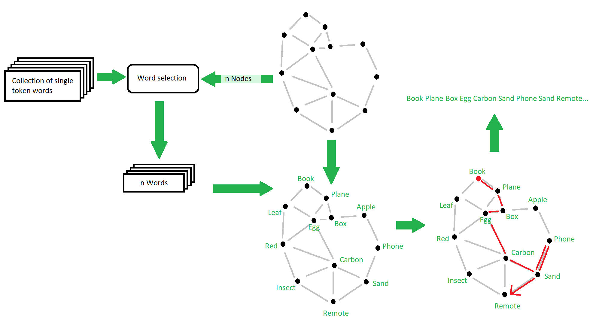
I create a dataset which first chooses a set of random words, one for each node in the graph. These words are chosen from a selection of words that each tokenize as a single token with Llama-3.1-8B’s tokenizer. After word selection, a random starting node on the graph is chosen and a random walk is started, appending the token associated with the current node for every step to the context. Figure 1 below shows this process.
Finding the representation:
[1] and [2] take the average of activations over the last 50 tokens and then average per token, however this means that A) the number of tokens averaged for each word is variable and B) they use dummy locations for words not yet seen. To fix these issues I simply average over the previous 4 tokens of each type, or all of the appearances if there are fewer than 4. If a word hasn’t appeared yet, I do not plot it or include it in the PCA. In my experiments this method gave more stable results in plotting, and being able to see when words are first seen and how that affects the representation is an interesting addition.
As in [1] and [2], I simply run PCA on activation averages and plot these averages in the 2D subspace spanned by the top 2 components.
Results:
To begin with I ran the experiment on 900 tokens, plotting for each position in the context (no different from doing a forward pass per new token, due to causal attention) on the original selection and placement of words on the 4x4 grid graph used in [1] and [2]. Figure 2 below is a plot of the evolution over time of the represenation in the 2D space found with PCA, clearly showing the geometric structure matching the 4x4 grid.
Other topologies:
Out of curiosity I tried a few novel graph topologies, and found that the model both learns to predict neighbors correctly, and represents them in a way recoverable with PCA. Figure 3a is interesting because it appears to be a 3D representation that we are projecting onto the top 2 PCA components. This suggests that, to some extent, the model constructs representations in whichever dimensionality is optimal for that particular topology.
Subspace analysis:
A natural question after finding this representation across multiple iterations is: are these all taking place in the same subspace? To test this, I collect the top 2 PCA components from 10 different repeats of the experiment with the fixed 4x4 configuration from [1], and then compute the chordal distance between each of these subspaces, as a metric of their similarity. I then repeat this for fixed word selection, randomized locations, and then for randomized word selection and locations. For reference, the average expected chordal distance between 2 randomly selected subspaces from a 4096 (residual stream width of the model) dimensional space is ~sqrt(2), or ~1.414.
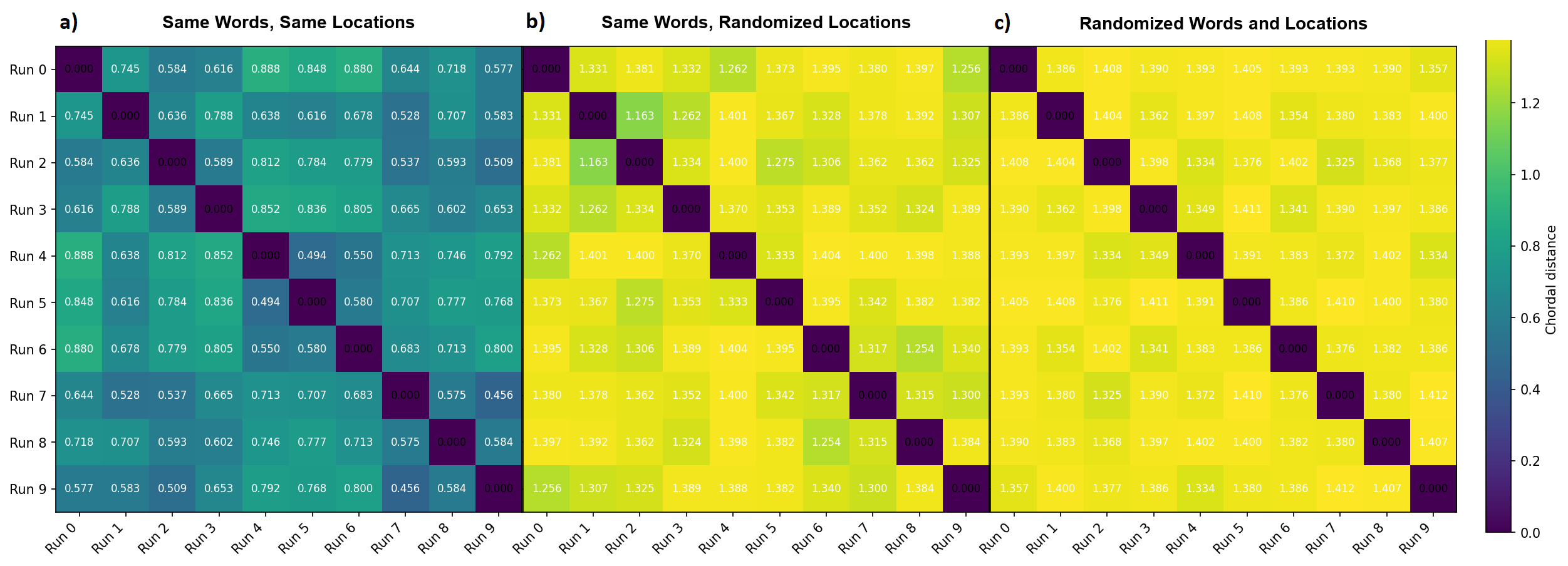
Figure 4a shows that with fixed word selection and locations, the subspaces are very similar, and Figure 4c shows that the subspaces are barely even related with randomized word selections and locations. We can explain the difference between 4a and 4c as a result of these representations being crafted as modifications to the embeddings of the tokens used, and so different tokens/embeddings should mean different subspaces. This theory predicts fixed word choices to always produce similarly aligned subspaces, but in Figure 4b, created using the same selection of words as 4a but random locations, the subspaces are barely aligned with each other. I did not expect this dependence on word locations. [2]’s results provide an explanation for this: the geometry comes primarily from neighbor mixing done by previous token attention heads, and so the locations in the residual stream are heavily dependent on which neighbors a word has.
Ablations:
To evaluate whether the representations I found are causally relevant for the task of outputting valid neighbors, I do ablations on the subspace we found them in and compare this to performance without the ablation. One complication here is that even in the case where the words chosen and their configuration in the grid are the same, the subspace that the representation lies in is not always the same, as seen in figure 4. To be able to do repeats with different random walks, I do a meta PCA, taking the top 2 components from all 10 experiments shown in figure 4, run PCA on that, and find that the top 3 components of this meta PCA explain 93.3% of the variation. This 3D subspace is what I ablate in the following experiment.
To test the effect of ablation, I create 10 different 1500 token long prompts, all using the same word selection and configuration, and then run the ablated and baseline model on these prompts, recording the validity of output at every token position in the prompt. These results are then averaged and plotted, with the baseline shown in blue, and the ablation shown in red, in figure 5 below. To test how much of an effect we get from this specific subspace being ablated, I also have a third regime where I ablate a randomly chosen 3D subspace in the residual stream, and compare this to the specific ablation and the baseline, this is shown in green.
The Y axis is the amount of probability mass assigned to the valid neighbors in the output logits of the model. For example, if apple only has valid neighbors bird and house in the graph, then assigning 0.5 to each gives a score of 1, while assigning 0.1 to bird and 0.2 to house gives a score of 0.3.
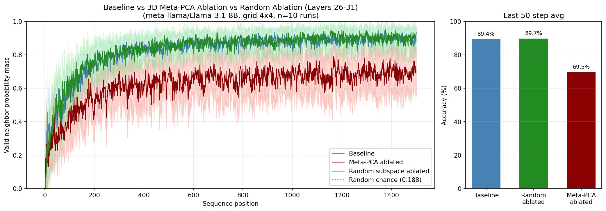
The baseline and random results are near identical, sitting at 89.4% and 89.7% respectively, while the ablation scores 69.5%, showing that the subspace ablated is causally relevant for the task, but that it isn’t critical / the only way the task is done. This could be because there are other similar representations in other subspaces, and that PCA is only surfacing one of these. Another way to look at this explanation is that the representations we are finding here actually have higher dimensional components that we aren’t ablating. For example in the left panel of figure 3, we seem to be looking at a 2D projection of a 3D representation, which is rotating relative to the subspace we are viewing (or vice versa).
Arditi 2026:
Arditi 2026 [2] suggests, in contrast to [1], that the geometry uncovered is simply an epiphenomenon created by the neighbor mixing that induction heads cause, and that the induction heads are what is really solving the task. Their evidence, besides a toy model showing that neighbor mixing alone produces the same geometry that we uncover through PCA, is that ablating the induction heads in the model destroys both performance and geometry.
My ablation of the subspace leads to a substantial performance drop, ~90% to ~70%, showing that the representations we are finding are causally relevant for performance. [2] finds that ablating the top 2 copy heads leads to a performance drop to 55%, and given that these copy heads should result in the kind of neighbor mixing that [2] describes, which should in turn create the geometric representations, it’s tempting to think that our subspace ablation result comes from simply ablating a part of what these copy heads do. To test this, I separately ablated the top 2 copy heads, the subspace, and then both at the same time (figure 6). Interestingly, the performance drop seems to stack, indicating that A) something other than these 2 copy heads is contributing to building the representation in the 2D subspace, and B) the 2 copy heads are contributing to performance in some other way than building the representation in this subspace. To further test this, following [2], I also ablate the top 32 copy heads, resulting in a reduction to 28% accuracy. I then combine the subspace ablation with the 32 head ablation, resulting in 20% accuracy, barely above the 18.8% random chance baseline.
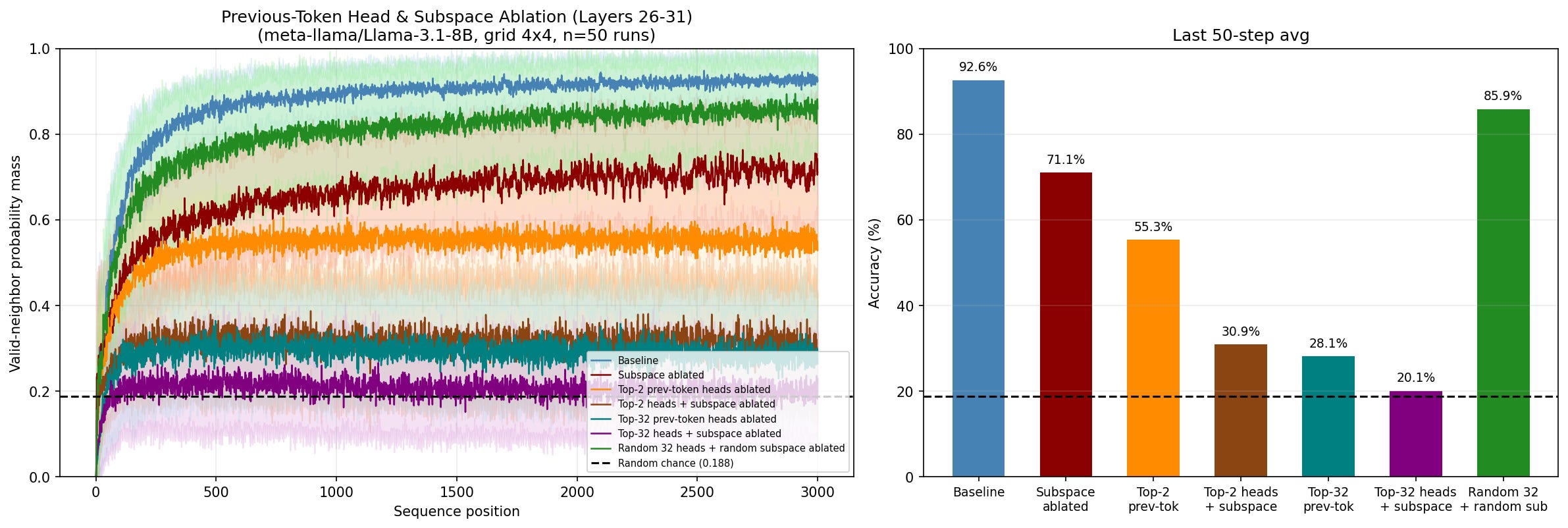
Figure 6 shows that the story is more complicated than that put forward in [2]: the copy heads are indeed responsible for most of the performance on the neighbor prediction task, but instead of the geometry found through PCA being an epiphenomenon, it is a significant part (but not all) of how the copy heads contribute to performance.
While my findings here do not tell a definitive story about the relationship between the representations we find through PCA and performance on the neighbor prediction task, they help bridge the gap between Park et al., 2025 [1] and Arditi 2026 [2], and will hopefully help contribute towards understanding the underlying mechanism in an incremental way.
Ekdeep gave a talk about this paper at Stanford